ZOAF
Towards Efficient Zeroth-Order Optimization for Analog/RF Circuit Design
Descent directions straight from the simulator. No surrogate, no adjoint.
1University of California, Santa Barbara2National Institute of Standards and Technology, Boulder
Overview
Gradient-style search for a simulator that gives no gradients.
Sizing an analog/RF circuit means tuning resistors, capacitors, device sizes and biases until gain, bandwidth, ripple or return loss meet their targets. Every candidate costs a SPICE or EM simulation, and commercial simulators expose no gradients, so adjoint-based optimization is off the table.
The usual answers each pay a price. Surrogate-based Bayesian optimization has to fit and tune a model of the circuit response; population heuristics such as CMA-ES, DE and PSO burn through the simulator budget. ZOAF takes a third route: it estimates descent directions from a handful of paired black-box simulations and takes gradient-style steps, with no surrogate and no simulator hooks.
Across an RF matching network and two amplifiers under equal simulator-call budgets, ZOAF reaches the best median final value on every reported figure of merit, has the most robust worst case across seeds, and matches each baseline's final median with 1.3–3.8× fewer simulator calls.
Method
Coarse random directions, then fine coordinates.
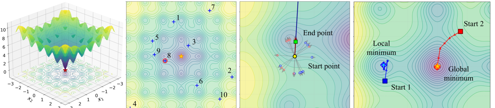
Each query runs the simulator at a design vector \(x\) inside its box \([\ell, u]\). ZOAF turns symmetric two-point probes into a gradient estimate, and chooses how to spend probes depending on how close the search is to a good basin.
Hybrid RGE → CGE
Random-direction estimation (RGE) costs \(2N\) calls per step and finds a promising basin cheaply. When progress slows, ZOAF switches to coordinate-wise estimation (CGE): \(2d\) calls, but low-variance and accurate for late-stage refinement.
One-shot multi-start
A single quasi-random pool (Sobol / LHS) is drawn and evaluated once, counted toward the budget. Restarts reuse it with a rank-based schedule: top designs first, lower ranks later for exploration.
Sliding-window monitor
Over the last \(W = 8\) steps it tracks improvement, gradient norm and trend. A soft stall shrinks the step and widens the probe; a hard stall ends the stage and restarts from the pool. Every probe and update is clipped to the box.
The RGE estimator is unbiased for the Gaussian-smoothed gradient, with smoothing bias \(O(L\mu\sqrt d)\) but mean-square error growing as \(O(d^2/N)\). That variance is what stalls RGE near an optimum, and what the switch to the deterministic, coordinate-wise CGE removes.
Playground
Watch the search spend its budget.
A two-parameter toy with a broad trap basin and a narrow, deeper optimum. ZOAF spends a few calls on a quasi-random pool, descends with cheap random-direction steps, refines with coordinate steps, and restarts when a stage stalls. Compare it with a run that never restarts, and with plain random sampling under the same budget.
22-parameter amplifier
Ahead early, and still ahead at the end.
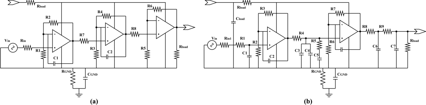
A two-stage cascaded signal-conditioning amplifier with 22 tunable components, three figures of merit to minimize, a 100-call budget and 100 random seeds per method. ZOAF has the best median on all three; on peaking its median is 5.7× lower than the best baseline.
Robust tails. On overshoot every baseline's worst seed lands between 15.2% and 21.2%, 2.5–3.4× above ZOAF's 6.15%. The 100-call budget is a saturated regime here: every median curve has flattened before call 100.
Three-stage op-amp
Top-left is where you want to be.
Ten passive components (\(R_{1..8}\), \(C_{1,2}\)), three figures of merit maximized one at a time under a 300-call budget. ZOAF ties the best DC gain in 72 calls instead of 200, and its gain–bandwidth product is ~180× that of CMA-ES — in about a second of runtime, where the GP-based methods take over 20 minutes.
RF matching network
Reliable, not just lucky once.
Fifteen lumped elements tuned for the deepest return loss \(|S_{22}|\) at 94 GHz, 150 calls, 10 runs per method. Below about −40 dB the engineering return diminishes, so the comparison that matters is the run-to-run mean.
Takeaway. GP-EI and GP-PI average −22.5 and −26.4 dB, short of the practical −30 dB threshold; GP-Mixer-AF barely clears −40 dB, and the strongest baseline, GASPAD, averages −45.8 dB. ZOAF averages −57.7 dB, with a tighter spread than GP-Mixer-AF.
FAQ
Questions people ask
What problem does ZOAF solve?
Optimizing analog and RF circuit parameters when the simulator is a black box, so gradients are unavailable and every evaluation is expensive.
Why not just use gradient-based optimization?
Classical gradient-based methods need access to simulator internals or an adjoint implementation. Commercial analog/RF simulators expose neither, so the gradient simply is not available.
How does ZOAF differ from Bayesian optimization, CMA-ES, or other black-box baselines?
Surrogate methods such as TuRBO, AutoCkt and DNN-Opt fit a model of the circuit response and optimize that model, which is expensive to build and sensitive to hyperparameters. Population heuristics such as CMA-ES, DE and PSO need many evaluations. ZOAF is surrogate-free: it estimates descent directions directly from a small number of simulations and takes gradient-style steps, converging with 1.3–3.8× fewer simulator calls.
What are the three main components?
A hybrid ZO schedule that switches between random-direction ZO for budget-efficient exploration and coordinate-wise ZO for accurate late-stage refinement; one-shot quasi-random multi-start to focus the evaluation budget; and a sliding-window monitor that triggers early stops and box-projected updates to keep parameters within feasible ranges.
What circuits was it evaluated on, and does it need simulator source code?
Three distinct schematics, including a 22-parameter two-stage cascaded amplifier where ZOAF shows up to an order-of-magnitude advantage in median peaking. It needs no source code — the simulator is treated strictly as a black box mapping design parameters to a figure of merit.
What comes next?
Extending the framework toward uncertainty-aware design: stochastic zeroth-order optimization to handle process variations in nanoscale circuits, and distributionally robust circuit optimization that accounts for distribution shift in those variations.
Citation
BibTeX
Abstract
Circuit optimization is an indispensable step in analog/RF IC design. Classical fast gradient-based optimization methods are typically infeasible due to lack of access to simulator source code and the technical barriers to implementing adjoint methods. Therefore, surrogate-based black-box optimization is widely used in practice; however, it can be costly to build and sensitive to hyperparameters, whereas population heuristics often suffer from slow convergence and large evaluation counts under tight simulator-call budgets. To address these limitations, we propose the Zeroth-Order Analog/RF Framework (ZOAF), which recovers gradient-descent directions from a small number of black-box circuit simulations, combining the benefits of both gradient-based optimization and black-box optimization. We also employ several surrogate-free techniques to improve the efficiency and accuracy, including (1) a hybrid ZO scheduling method that switches between random-direction ZO for budget-efficient exploration and coordinate-wise ZO for accurate late-stage refinement, (2) one-shot quasi-random multi-start to focus evaluations, and (3) a sliding-window monitor that triggers early stops and box-projected updates to maintain feasibility. Evaluated on three distinct schematics, ZOAF consistently outperforms state-of-the-art baselines, achieving the best median final value on every reported figure of merit — with up to an order-of-magnitude advantage in median peaking on the 22-parameter two-stage amplifier — together with the most robust worst-case behavior across seeds, while reducing simulator calls to convergence by 1.3–3.8×.
@article{tan2026zoaf,
  title   = {ZOAF: Towards Efficient Zeroth-Order Optimization for Analog/RF Circuit Design},
  author  = {Tan, Liyan and Zhao, Yequan and Lu, Jinming and Jamroz, Ben F. and Feldman, Ari and Zhang, Zheng},
  journal = {arXiv preprint arXiv:2606.02869},
  year    = {2026}
}