Simulation-Efficient Analog Circuit Yield Optimization via Monte Carlo Zeroth-Order Gradient Estimation

Q: How is the gradient estimated, and why is it cheap?

At each step the design is perturbed along K random Gaussian directions in plus/minus pairs, with the process realization held fixed inside each pair so the difference isolates the design perturbation rather than process noise. The K differences are averaged into one stochastic gradient at a cost of 2K = 8 SPICE simulations. For comparison, the direct-yield baselines spend ten simulations to estimate one scalar yield — eight simulations buy a direction in design space instead.

Q: How does it compare with Bayesian optimization, CMA-ES, PSO, TuRBO and RobustAnalog?

All six methods run under the same per-run SPICE budget rather than the same iteration count. ZO-MC-SGD ties the best baseline on the two easiest circuits and needs four to eight times less budget on the other three. An ablation reruns BO, CMA-ES, PSO and TuRBO on the softplus surrogate as well: direct yield is better for all four on every circuit, by 0.24–0.41 mean yield on average, so the baselines are reported on the objective that favors them.

Q: Does it need the process variables to be independent?

No — only independent samples from their joint distribution. Replacing the independent process model with a correlated one (correlation 0.5 among parameters sharing oxide, doping or lithographic effects) leaves the advantage intact: 200 simulations to target on 3-stage csamp against 400 for CMA-ES, and 25 against 100 on 2-stage csmiller.

Q: What are the limits, and what comes next?

The method needs a process distribution that can be sampled. If that distribution is itself uncertain or drifts across manufacturing conditions, the problem becomes optimization under distributional uncertainty, and a distributionally robust formulation is the natural extension. The bounds carry no explicit process-dimension term, but the experiments only reach 42 mismatch variables; production-scale circuits with hundreds may need variance reduction or structure-exploiting estimators.

Liyan Tan; Yequan Zhao; Ben F. Jamroz; Ari Feldman; Zheng Zhang

doi:10.48550/arXiv.2609.30678

Under review

ZO-MC-SGD

Simulation-Efficient Analog Circuit Yield Optimization via Monte Carlo Zeroth-Order Gradient Estimation

Eight SPICE runs buy a direction, not a single yield number.

Liyan Tan¹ Yequan Zhao¹ Ben F. Jamroz² Ari Feldman² Zheng Zhang¹

¹University of California, Santa Barbara²National Institute of Standards and Technology, Boulder

Paper arXiv Code BibTeX

8×fewer SPICE simulations than the best baseline (5-stage csamp)

50–200SPICE simulations to a 0.95 mean yield, on all five benchmarks

8SPICE runs per descent direction (2K, K = 4)

48 msoptimizer overhead at 30 design variables (BO: 464 s)

Overview

Optimize the margins, score the yield.

A fabricated analog circuit only ships if it meets every specification under process variation. That probability, the yield, is what makes a design manufacturable — but every candidate has to be checked across many Monte Carlo SPICE samples, and the finite-sample estimate barely moves when the design does.

ZO-MC-SGD keeps yield as the score and changes the optimization signal. Each SPICE run is turned into continuous specification margins, a softplus loss is checked for rank agreement with yield, and paired design perturbations under shared process samples give a stochastic descent direction — no SPICE derivatives, no global surrogate model.

TL;DR

Across five SPICE benchmarks with up to 30 design and 42 process variables, ZO-MC-SGD reaches a 0.95 mean yield within 50–200 simulations. It ties the best of five black-box and learning-based baselines on the two easiest circuits and needs 4–8× fewer simulations on the other three.

Why

Yield is flat. Margins are not.

With a fixed set of process samples, the yield estimate only changes when a sample crosses a specification boundary, so it is piecewise constant and its local slope is zero almost everywhere. The margins behind it vary smoothly, and a softplus loss built from them keeps pointing the way.

One design knob, two specifications Toy model

Gain improves and power worsens as the knob increases; each sample adds Gaussian process noise to both margins. Hover the plots to probe a design. An illustration of the idea, not circuit data.

Yield estimate Ŷthe score

Softplus margin lossthe optimization signal

Sharpness α6

Knob x–

Ŷ(x)–

Local slope of Ŷ–

Local slope of loss–

Rank check ρ_saccept if ≤ −0.7–

Method

From a SPICE run to a descent direction.

ZO-MC-SGD minimizes the expected per-sample loss $F(x)=\mathbb{E}_{\xi\sim\rho}[\ell(x,\xi)]$ over the design box, while the yield $Y(x)$ stays the quantity used to judge the returned design.

1

Margins, not pass/fail

Gain (dB), unity-gain bandwidth (decades of Hz) and power (mW) become signed shortfalls $\delta_k$ against their specs. A softplus with sharpness $\alpha_k$ penalizes violations and keeps rewarding margin near the boundary.

2

Check the ordering

Before optimizing, the Spearman rank correlation between mean loss and empirical yield is measured on 81 perturbed designs. The loss is used only if $\rho_s \le -0.7$; all five circuits pass, at −0.873 to −0.977.

3

Paired perturbations

Each of $K = 4$ random directions is probed at $x \pm \epsilon v$ under the same process sample, so the difference isolates the design change. 2K = 8 SPICE runs give one gradient estimate, followed by a projected Adam step.

$$\sigma_k = \frac{1}{\alpha_k}\log\!\bigl(1+e^{\alpha_k\delta_k(x,\xi)}\bigr), \qquad \ell(x,\xi) = \sum_k w_k\,\sigma_k - \gamma\, f_{\text{gain}}(x,\xi)$$

$$\hat g^{\,\text{MC}} = \frac{1}{K}\sum_{i=1}^{K}\frac{\ell\bigl(x+\epsilon v^{(i)},\xi^{(i)}\bigr)-\ell\bigl(x-\epsilon v^{(i)},\xi^{(i)}\bigr)}{2\epsilon}\,v^{(i)}, \qquad x \leftarrow \Pi_{[0,1]^n}\bigl(x-\eta\,\hat g^{\,\text{MC}}\bigr)$$

What a SPICE run buys: the direct-yield baselines (BO, CMA-ES, PSO, TuRBO) spend 10 simulations per query to estimate one scalar yield; RobustAnalog spends 20 per step on its margin reward; ZO-MC-SGD spends 8 to estimate a direction in design space. All methods share the same per-run SPICE budget, including ZO-MC-SGD’s random-search warm start.

Results

The gap widens as circuits grow.

Five circuits, eight budgets from 25 to 3,200 SPICE runs, five seeds each; every returned design is re-scored on the same 80 held-out process samples. The competing methods must first fit a model, evaluate a population or train a policy; ZO-MC-SGD turns each 8-run batch straight into a step.

Mean yield vs. SPICE budget: hover to compare

Five-seed mean yield, best so far over budgets as in the paper’s figure; the dashed line is the 0.95 target, and “0” is the shared initial design. Click a baseline on the right to highlight it.

ZO-MC-SGDselected baselineother baselines

Takeaway. On the 3- and 5-stage CS cascades the strongest baselines need 800 simulations where ZO-MC-SGD needs 200 and 100. CMA-ES never reaches the target on 3-stage csamp, and RobustAnalog misses it on three of five circuits even at 3,200.

Checks

Aligned, re-scored, and fair to the baselines.

Three questions a skeptical reader should ask: does lower loss really mean higher yield, does the returned yield survive a much larger fresh sample, and would the baselines have done better on the same surrogate?

Rank alignment ρ_saccept ≤ −0.7

Yield on 1000 fresh samplestarget 0.95

Direct yield − softplusbaselines

Left: Spearman correlation between mean loss and empirical yield on the 81-design calibration set. Middle: ZO-MC-SGD designs returned at the target budgets, re-estimated with N = 1000; dot = five-seed mean, bar = observed range. On CS ×1 no method exceeds 0.95 at any budget, an empirical yield ceiling. Right: rerunning BO, CMA-ES, PSO and TuRBO on the softplus surrogate makes every one of them worse on every circuit (bar: mean over circuits, dots: individual circuits), so the main comparison uses direct yield for them. Hover for exact values.

Also robust to correlated variation. With 0.5 correlation among parameters sharing oxide, doping or lithographic effects, ZO-MC-SGD still needs 200 simulations on 3-stage csamp (CMA-ES: 400) and 25 on 2-stage csmiller (CMA-ES: 100). It needs independent samples, not independent process variables.

Cost

The optimizer itself is almost free.

SPICE takes about 350 s for every method at a 1,600-run budget. What differs is the optimizer’s own computation, which grows with the design dimension for the surrogate-model methods.

Theory

No explicit dependence on the process dimension.

1

Unbiased

The estimator is unbiased for the gradient of the Gaussian-smoothed objective $F_\epsilon$, which differs from $F$ by $O(\epsilon^2)$.

2

Variance ∝ 1/K

Its variance falls as $1/K$ with no explicit factor of the process dimension; process variation enters only through the per-sample gradient variance.

3

Sample complexity

Reaching $\nu$-stationarity takes $O(n/\nu^2)$ SPICE evaluations, independent of the mini-batch size and of the process dimension.

The estimator, checked against ground truth

Normalized error of the averaged estimate against the number of independent estimates M, at the deployed K = 4 and ε = 5×10⁻³ (n = 6, d_ξ = 10). Bars are 95% bootstrap intervals; the dashed line is the M^−1/2 rate.

S1 · stochastic quadraticexact gradient

S2 · softplus, yield-like2×10⁶-sample reference

Both follow the M^−1/2 sampling rate; S2 reaches 0.57% at M = 1.28×10⁵. Varying ε over a fourfold range shows no bias floor, consistent with the O(ε²) smoothing error.

Benchmarks

Five circuits, two families.

Common-source cascades with one, three and five stages, and Miller-compensated amplifiers with two and three, simulated in ngspice with Pelgrom-scaled Gaussian device mismatch. A sample passes only when gain, unity-gain bandwidth and static power all meet their limits at once (V_DD = 1 V).

Circuit	n	d_ξ	Gain	UGBW	Power	Initial yield	ρ_s
1-stage csamp	6	10	≥ 20 dB	≥ 1.0 MHz	≤ 0.5 mW	0.24	−0.977
3-stage csamp	18	26	≥ 60 dB	≥ 50 MHz	≤ 0.5 mW	0.20	−0.873
5-stage csamp	30	42	≥ 95 dB	≥ 30 MHz	≤ 0.7 mW	0.34	−0.915
2-stage csmiller	14	26	≥ 50 dB	≥ 0.2 MHz	≤ 0.5 mW	0.64	−0.876
3-stage csmiller	22	38	≥ 60 dB	≥ 0.05 MHz	≤ 0.7 mW	0.66	−0.953

One-stage common-source amplifier schematic

Two-stage Miller-compensated amplifier schematic

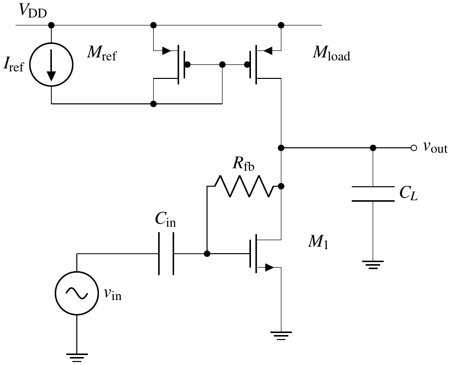
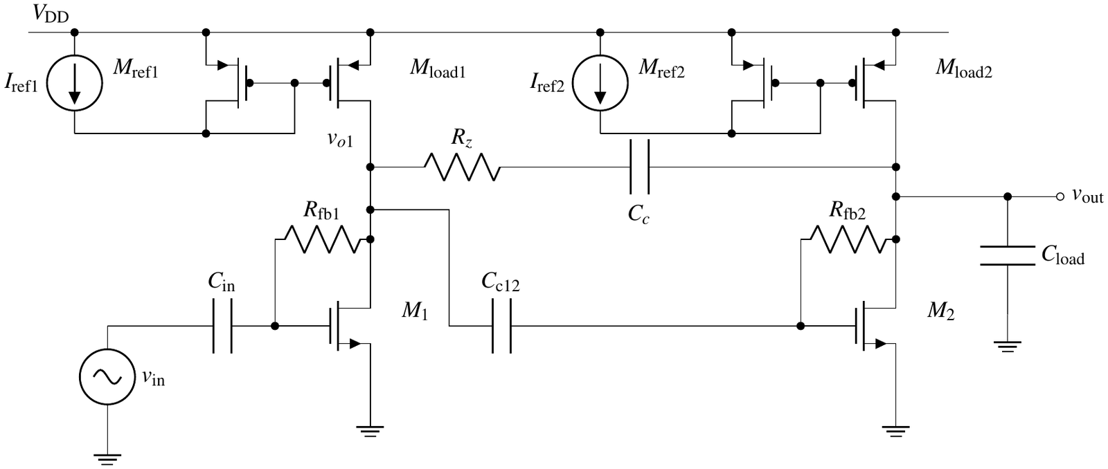
The base topology of each family: a common-source stage (left) and a two-stage Miller-compensated amplifier (right). n is the design dimension and d_ξ the number of process variables.

FAQ

Questions people ask

What problem does ZO-MC-SGD solve?

Sizing an analog circuit so that it meets all of its specifications under process variation, not just at the nominal operating point — that is, maximizing yield — when SPICE is a black box and the simulation budget is only a few hundred runs.

Why not just run a black-box optimizer on the Monte Carlo yield estimate?

Because with a fixed set of process samples the estimate only changes when a sample crosses a specification boundary, so it is piecewise constant over large regions and carries no local direction. Its accuracy also improves only as N^(-1/2), so a reliable estimate is expensive, and each one buys a single scalar at a single design point.

What is the yield-aligned loss, and how do you know it is aligned?

Every metric is scaled to comparable units, turned into a signed margin against its specification, and passed through a softplus whose sharpness controls how far past the boundary the metric keeps influencing the loss; the penalties are then combined with weights plus a mild preference for gain headroom. Alignment is checked, not assumed: the Spearman rank correlation between mean loss and empirical yield is measured on a fixed calibration set of 81 perturbed designs and the loss is accepted only at rho_s <= -0.7. All five benchmarks pass, from -0.873 to -0.977.

How is the gradient estimated, and why is it cheap?

At each step the design is perturbed along K random Gaussian directions in plus/minus pairs, with the process realization held fixed inside each pair so the difference isolates the design perturbation rather than process noise. The K differences are averaged into one stochastic gradient at a cost of 2K = 8 SPICE simulations. For comparison, the direct-yield baselines spend ten simulations to estimate one scalar yield — eight simulations buy a direction in design space instead.

What does the theory guarantee?

The estimator is unbiased for the gradient of the Gaussian-smoothed objective, with an O(eps^2) discrepancy from the unsmoothed one. Its variance falls as 1/K and carries no explicit factor in the process dimension — process variation enters only through the per-sample gradient variance. Reaching nu-stationarity takes O(n/nu^2) SPICE evaluations, independent of the mini-batch size and of the process dimension. Synthetic problems with analytic reference gradients confirm the predicted M^(-1/2) error decay.

How does it compare with Bayesian optimization, CMA-ES, PSO, TuRBO and RobustAnalog?

All six methods run under the same per-run SPICE budget rather than the same iteration count. ZO-MC-SGD ties the best baseline on the two easiest circuits and needs four to eight times less budget on the other three. An ablation reruns BO, CMA-ES, PSO and TuRBO on the softplus surrogate as well: direct yield is better for all four on every circuit, by 0.24–0.41 mean yield on average, so the baselines are reported on the objective that favors them.

Does it need the process variables to be independent?

No — only independent samples from their joint distribution. Replacing the independent process model with a correlated one (correlation 0.5 among parameters sharing oxide, doping or lithographic effects) leaves the advantage intact: 200 simulations to target on 3-stage csamp against 400 for CMA-ES, and 25 against 100 on 2-stage csmiller.

What are the limits, and what comes next?

The method needs a process distribution that can be sampled. If that distribution is itself uncertain or drifts across manufacturing conditions, the problem becomes optimization under distributional uncertainty, and a distributionally robust formulation is the natural extension. The bounds carry no explicit process-dimension term, but the experiments only reach 42 mismatch variables; production-scale circuits with hundreds may need variance reduction or structure-exploiting estimators.

Citation

BibTeX

Abstract

Yield optimization under process variation is expensive because each candidate design must be evaluated across many Monte Carlo SPICE samples. The resulting finite-sample yield is also piecewise constant in the design parameters, providing little local information for optimization. We introduce zeroth-order Monte Carlo stochastic gradient descent (ZO-MC-SGD), a black-box method that converts continuous specification margins into stochastic descent directions. Each update evaluates opposite design perturbations under shared process samples, allowing a small simulation batch to estimate a local direction without differentiating SPICE or fitting a global surrogate model. A Spearman rank-correlation test checks that the margin-based loss orders designs consistently with empirical yield. We prove that the estimator is unbiased for a Gaussian-smoothed surrogate and derive variance and sample-complexity bounds with no explicit dependence on process dimension. Across five analog circuit benchmarks with up to 30 design variables and 42 process variables, ZO-MC-SGD reaches a mean yield of 0.95 on four circuits within 50–200 simulations and the empirical yield ceiling on the fifth. Relative to the best of five black-box and learning-based baselines, it reduces the required simulation budget by up to a factor of eight.

@article{tan2026yield,
  title   = {Simulation-Efficient Analog Circuit Yield Optimization via Monte Carlo Zeroth-Order Gradient Estimation},
  author  = {Tan, Liyan and Zhao, Yequan and Jamroz, Ben F. and Feldman, Ari and Zhang, Zheng},
  journal = {arXiv preprint arXiv:2609.30678},
  year    = {2026}
}